Overview
Species distribution modeling (SDM) predicts where plants can survive under different climate conditions. The API uses MaxEnt algorithms with CHELSA climate data to generate distribution maps for current and future scenarios.How it works
The modeling process combines species occurrence records with environmental variables to predict habitat suitability. The system downloads occurrence data from GBIF (Global Biodiversity Information Facility), processes climate data at 1-kilometer resolution, and generates suitability maps using maximum entropy modeling.Data sources
The API uses two primary data sources: Species occurrence records: Downloaded from GBIF using taxonomy-resolved searches that include synonyms. The system fetches up to 20,000 records per species and requires at least 30 occurrence points for MaxEnt modeling. Species with fewer records use simplified niche modeling. Climate data: CHELSA version 2.1 provides all 19 bioclimatic variables at 1-kilometer resolution, covering temperature and precipitation patterns. Data is available for the historical baseline (1981-2010) and future projections. Automated variable selection reduces these to the most informative subset (typically 5-8 variables) by removing highly correlated pairs and multicollinear predictors.Climate scenarios
Future projections use CMIP6 climate models with four emission scenarios:- SSP1-2.6: Low emissions scenario with strong mitigation
- SSP2-4.5: Intermediate emissions scenario
- SSP3-7.0: High emissions scenario with limited mitigation
- SSP5-8.5: Very high emissions scenario without mitigation
Output types
The API generates four visualization types:Suitability change map
Shows areas of habitat gain, loss, and stability between current and future climates. Green indicates stable suitable habitat, red shows habitat loss, blue represents new suitable areas, and gray marks consistently unsuitable regions.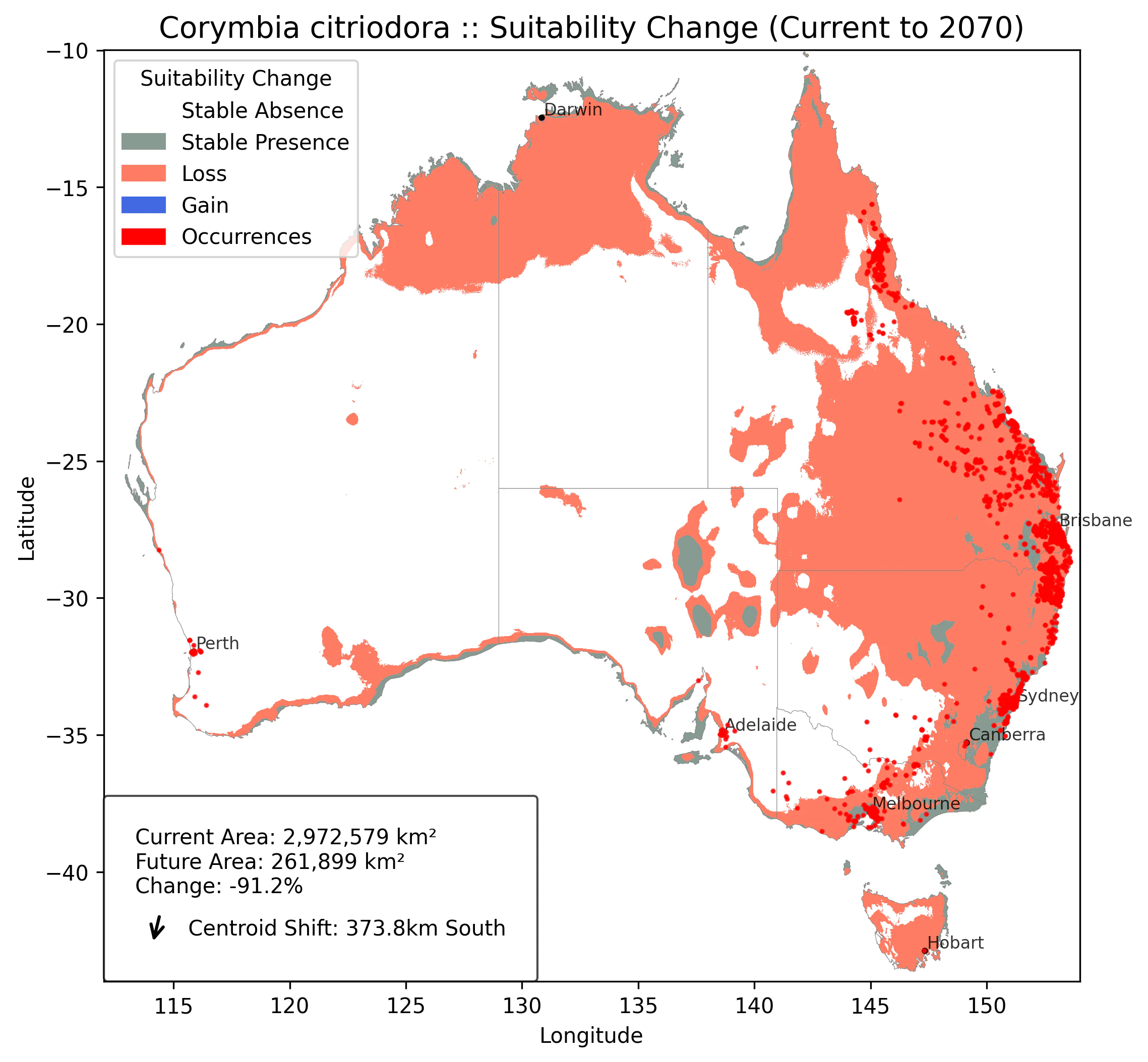
Current gradient map
Displays current climate suitability using a gradient from low (light) to high (dark) suitability. Occurrence points appear as red dots overlaid on the suitability surface.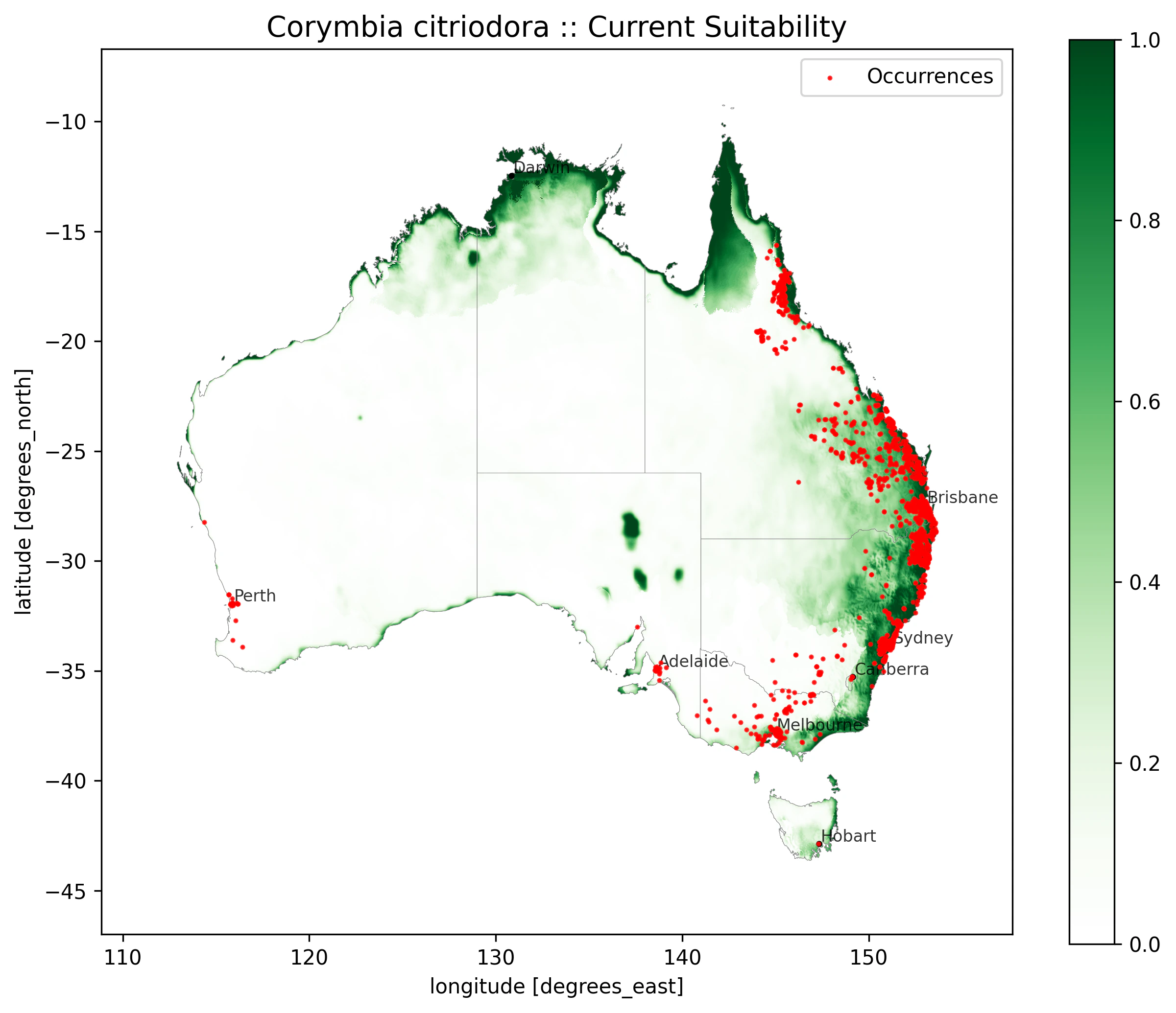
Future gradient map
Shows predicted suitability for the selected future period and scenario using the same gradient scale as the current map.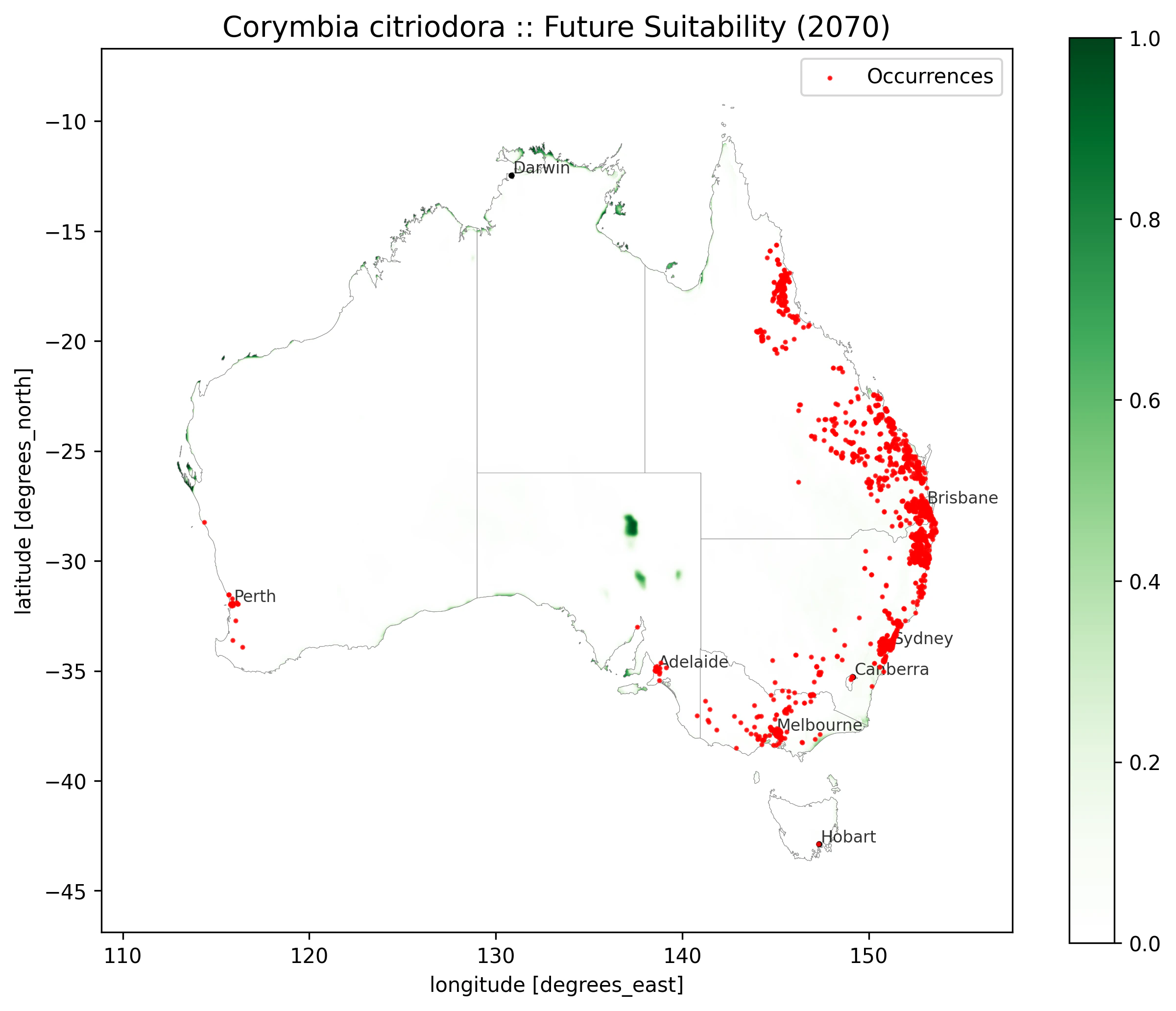
Trajectory streamplot
Visualizes habitat shift patterns using streamlines. The flow field shows the direction and magnitude of suitable habitat movement over time. Darker streamlines indicate stronger directional shifts.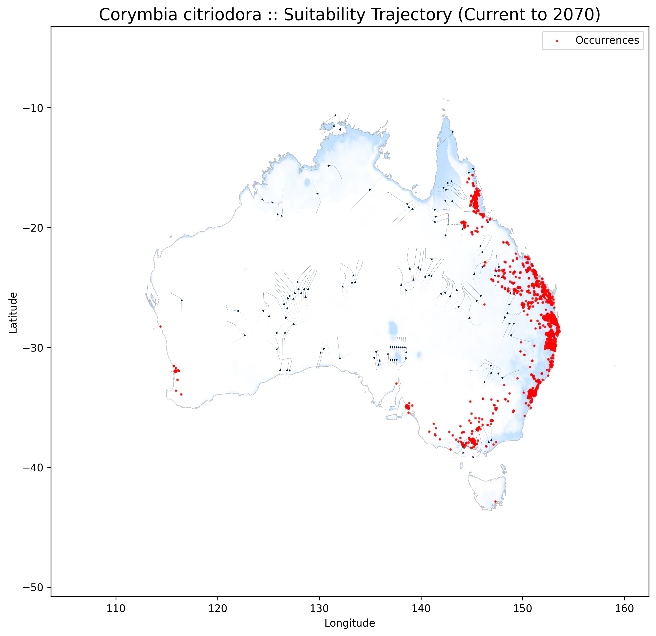
Use cases
SDM supports several conservation and planning applications: Conservation planning: Identify climate refugia where species are likely to persist. These stable areas become priorities for habitat protection. Restoration site selection: Locate areas that will become suitable in the future. These sites are candidates for assisted migration or pre-emptive planting. Risk assessment: Evaluate vulnerability of existing plantings to climate change. Areas showing habitat loss require adaptation strategies. Species selection: Choose climate-resilient species for landscaping projects. Species with expanding suitable habitat are better long-term choices.Limitations
Several factors affect model accuracy: Data quality: Models depend on occurrence record quality and completeness. Species with limited observations or biased sampling produce less reliable predictions. Climate variables: The model uses bioclimatic variables derived from temperature and precipitation. Soil type, topography, and land use are not currently included. Dispersal capacity: Models assume species can reach all suitable habitat. Natural dispersal limitations and barriers are not considered. Biotic interactions: Competition, pollination, and other species interactions are not modeled. These factors can prevent establishment in otherwise suitable habitat.API workflow
The typical workflow involves three steps:- Submit a modeling request with species name and climate scenario
- Poll the status endpoint until processing completes (typically 2-4 minutes)
- Download the generated visualizations
Best practices
For reliable results:- Use full scientific names including genus and species
- Select climate models appropriate for your region (MPI-ESM1-2-HR performs well globally)
- Consider multiple scenarios to bracket uncertainty
- Validate results against local knowledge and field observations
- Combine SDM outputs with other decision factors